
Файл:Partial transmittance.gif
Не е налична версия с по-висока разделителна способност.
Partial_transmittance.gif (367 × 161 пиксела, големина на файла: 67 КБ, MIME-тип: image/gif, зациклен, 53 кадъра, 4,2 сек)
| Този файл е от Общомедия и може да се използва от други проекти.
Следва информация за файла, достъпна през оригиналната му описателна страница. |
Резюме
| Описание |
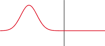
Русский: Показано классическое отражение/прохождение солитона гауссового импульса от/в более плотную среду. В реальности же, свет отражается не от поверхности, а от всех частиц тела (см. ru:КЭД). English: Illustration of partial reflection of a wave. A gaussian wave on a one-dimensional string strikes a boundary with transmission coefficient of 0.5. Half the wave is transmitted and half is reflected.
Français : Illustration de la réflection partielle d'une onde. Une onde gaussienne se déplaçant sur un ressort unidimensionnel est réfléchie/transmise au niveau d'une interface avec un coefficient de transmission de 0.5.
Español: Ilustración de una reflexión parcial de una onda. Una onda gaussiana sobre una cuerda de una dimensión choca contra un limite con un coeficiente de transmisión de 0.5. La mitad de la onda es transmitida y la otra mitad es reflejada. |
| Дата | |
| Източник | self-made with MATLAB, source code below |
| Автор | Oleg Alexandrov |
This diagram was created with MATLAB.
Лицензиране
| Аз, носителят на авторските права над тази творба, я публикувам като обществено достояние. Това разрешение е в сила за целия свят. В някои държави това може да не е възможно от законодателна гледна точка; затова: Давам на всекиго правото да използва тази творба за всякакви цели, без никакви условия, освен ако такива условия съществуват по закон. |
MATLAB source code
% Partial transmittance and reflectance of a wave
% Code is messed up, don't have time to clean it now
function main()

   % KSmrq's colors
   red    = [0.867 0.06 0.14];
   blue   = [0, 129, 205]/256;
   green  = [0, 200,  70]/256;
   yellow = [254, 194,   0]/256;
   white = 0.99*[1, 1, 1];
   black = [0, 0, 0];

   % length of the string and the grid
   L = 5;
   N = 151;
   X=linspace(0, L, N);

   h = X(2)-X(1); % space grid size
   c = 0.01; % speed of the wave
   tau = 0.25*h/c; % time grid size

   % form a medium with a discontinuous wave speed
   C = 0*X+c;

   D=L/2;
   c_right = 0.5*c; % speed to the right of the disc
   for i=1:N
      if X(i) > D
         C(i) = c_right;
      end
   end
   % Now C = c for x < D, and C=c_right for x > D

   K = 5; % steepness of the bump
   S = 0; % shift the wave
   f=inline('exp(-K*(x-S).^2)', 'x', 'S', 'K'); % a gaussian as an initial wave
   df=inline('-2*K*(x-S).*exp(-K*(x-S).^2)', 'x', 'S', 'K'); % derivative of f

   % wave at time 0 and tau
   U0 = 0*f(X, S, K);
   U1 = U0 - 2*tau*c*df(X, S, K);

   U = 0*U0; % current U

   % plot between Start and End
   Start=130; End=500;

   % hack to capture the first period of the wave
   min_k = 2*N; k_old = min_k; turn_on = 0;

   frame_no = 0;
   for j=1:End

      %  fixed end points
      U(1)=0; U(N)=0;

      % finite difference discretization in time
      for i=2:(N-1)
         U(i) = (C(i)*tau/h)^2*(U1(i+1)-2*U1(i)+U1(i-1)) + 2*U1(i) - U0(i);
      end

      % update info, for the next iteration
      U0 = U1; U1 = U;

      spacing=7;

     % plot the wave
      if rem(j, spacing) == 1 & j > Start

         figure(1); clf; hold on;
         axis equal; axis off;
         lw = 3; % linewidth

         % size of the window
         ys = 1.2;

         low = -0.5*ys;
         high = ys;
         plot([D, D], [low, high], 'color', black, 'linewidth', 0.7*lw)
%         fill([X(1), D, D, X(1)], [low, low, high, high], [0.9, 1, 1], 'edgealpha', 0);
%         fill([D X(N), X(N), D],  [low, low, high, high], [1, 1, 1], 'edgealpha', 0);

         plot(X, U, 'color', red, 'linewidth', lw);

         % plot the ends of the string
         small_rad = 0.06;

         axis([-small_rad, 0.82*L, -ys, ys]);

         % small markers to keep the bounding box fixed when saving to eps
         plot(-small_rad, ys, '*', 'color', white);
         plot(L+small_rad, -ys, '*', 'color', white);

         pause(0.1)
         frame_no = frame_no + 1;
         %frame=sprintf('Frame%d.eps', 1000+frame_no); saveas(gcf, frame, 'psc2');
         frame=sprintf('Frame%d.png', 1000+frame_no);% saveas(gcf, frame);
         disp(frame)
         print (frame, '-dpng', '-r300');

      end
   end


% The gif image was creating with the command
% convert -antialias -loop 10000  -delay 8 -compress LZW -scale 20% Frame10*png Partial_transmittance.gif
% and was later cropped in Gimp
История на файла
Избирането на дата/час ще покаже как е изглеждал файлът към онзи момент.
| Дата/Час | Миникартинка | Размер | Потребител | Коментар | |
|---|---|---|---|---|---|
| текуща | 16:36, 9 април 2010 | | 367 × 161 (67 КБ) | Aiyizo | optimized animation |
| 05:56, 26 ноември 2007 |  | 367 × 161 (86 КБ) | Oleg Alexandrov | {{Information |Description=Illustration of en:Transmission coefficient (optics) |Source=self-made with MATLAB, source code below |Date=~~~~~ |Author= Oleg Alexandrov |Permission=PD-self, see below |other_versions= }} {{PD-se |
Използване на файла
Следната страница използва следния файл:
Глобално използване на файл
Този файл се използва от следните други уикита:
- Употреба в ar.wikipedia.org
- Употреба в ca.wikipedia.org
- Употреба в de.wikipedia.org
- Reflexion (Physik)
- Fresnelsche Formeln
- Zeitbereichsreflektometrie
- Anpassungsdämpfung
- Benutzer Diskussion:Bleckneuhaus
- Wikipedia Diskussion:WikiProjekt SVG/Archiv/2012
- Wellenwiderstand
- Benutzer:Ariser/Stehwellenverhältnis Alternativentwurf
- Benutzer:Herbertweidner/Stehwellenverhältnis Alternativentwurf
- Benutzer:Physikaficionado/Fresnelsche Formeln-Röntgenstrahlung
- Употреба в de.wikibooks.org
- Употреба в en.wikipedia.org
- Употреба в en.wikibooks.org
- Употреба в en.wikiversity.org
- Quantum mechanics/Timeline
- How things work college course/Quantum mechanics timeline
- Quantum mechanics/Wave equations in quantum mechanics
- MATLAB essential/General information + arrays and matrices
- WikiJournal of Science/Submissions/Introduction to quantum mechanics
- WikiJournal of Science/Issues/0
- Talk:A card game for Bell's theorem and its loopholes/Conceptual
- Wright State University Lake Campus/2019-1/Broomstick
- Physics for beginners
- MyOpenMath/Physics images
- Употреба в es.wikipedia.org
- Употреба в et.wikipedia.org
- Употреба в fa.wikipedia.org
- Употреба в fa.wikibooks.org
- Употреба в fr.wikipedia.org
- Употреба в he.wikipedia.org
- Употреба в hy.wikipedia.org
Преглед на глобалната употреба на файла.